Numpy : calcul vectoriel en Python

Conventions

>>> import numpy as np
>>> import scipy as sp
>>> import pylab as pl

Le calcul avec des tableaux

Python	numpy
List: a = [1, 2, 3]	Tableau: a = np.array([1, 2, 3])

Faire des opérations sur beaucoup de nombres

• Calcul numérique classique = boucles

  def square(data):
      for i in range(len(data)):
          data[i] = data[i]**2
      return data
  

  In [1]: %timeit data = range(1000) ; square(data)
  1000 loops, best of 3: 314 us per loop
  

• Calcul vectoriel: remplacer les boucles par des opérations sur des tableaux

  def square(data):
      return data**2
  

  In [2]: %timeit data=np.arange(1000) ; square(data)
  100000 loops, best of 3: 10.6 us per loop
  

  Bénéfice du polymorphisme: même code pour un seul nombre, ou un tableau.

Des objets multi-dimensionels

>>> a = np.arange(10)
>>> a
array([0, 1, 2, 3, 4, 5, 6, 7, 8, 9])
>>> b = np.reshape(a, (2, 5))
>>> b
array([[0, 1, 2, 3, 4],
       [5, 6, 7, 8, 9]])
>>> b[:, 1]
array([1, 6])

Création de tableaux

• Création avec des constantes:

  >>> np.ones((2, 3))
  array([[ 1.,  1.,  1.],
         [ 1.,  1.,  1.]])
  

• Les tableaux contienent des entrées typées uniformement:

  >>> np.ones(3, dtype=np.int)
  array([1, 1, 1])
  

• Création d’une grille:

  >>> x, y = np.indices((2, 2))
  >>> x
  array([[0, 0],
         [1, 1]])
  >>> y
  array([[0, 1],
         [0, 1]])
  >>> x+1j*y
  array([[ 0.+0.j,  0.+1.j],
         [ 1.+0.j,  1.+1.j]])
  

Slicing

Parcourt multidimensionel des tableaux

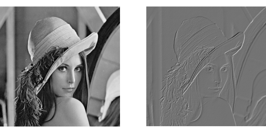
Un exemple d’application: calcul du laplacien

image[1:-1, 1:-1] = (image[:-2, 1:-1] - image[2:, 1:-1] +
                     image[1:-1, :-2] - image[1:-1, 2:])*0.25

In [3]: import pylab as pl
In [4]: l = sp.lena()
In [5]: pl.imshow(l, cmap=pl.cm.gray())
In [6]: e = l[:-2, 1:-1] - l[2:, 1:-1] + l[1:-1, :-2] - l[1:-1, 2:]
In [7]: pl.imshow(e, pl.cm.gray())

---

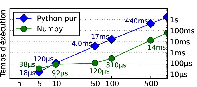
Gains en temps

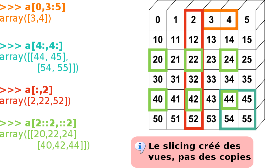
Indexage avancé

Avec des entiers ou des masques

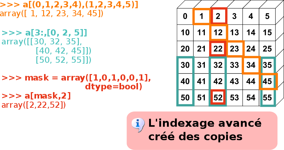
Utilisation de tableaux d’entiers

• Trier un vecteur avec un autre:

  >>> a, b = np.random.random_integers(10, size=(2, 4))
  >>> a
  array([8, 6, 2, 9])
  >>> b
  array([ 8,  9,  3, 10])
  >>> a_order = np.argsort(a)
  >>> a_order
  array([2, 1, 0, 3])
  >>> b[a_order]
  array([ 3,  9,  8, 10])
  

Utilisation de masques

• Mettre tous les éléments pair d’un tableau à zéro:

  >>> a = np.arange(10)
  >>> a
  array([0, 1, 2, 3, 4, 5, 6, 7, 8, 9])
  >>> a[a % 2] = 0
  >>> a
  array([0, 0, 2, 3, 4, 5, 6, 7, 8, 9])
  

• Masque à partir d’une grille pour selectionner le centre de l’image:

  In [8]: n, m = l.shape
  In [9]: x, y = np.indices((n, m))
  In [10]: distances = np.sqrt((x - 0.5*n)**2 + (y - 0.5*m)**2)
  In [11]: l[distance > 200] = 255
  In [12]: pl.imshow(l, cmap=pl.cm.gray)
  

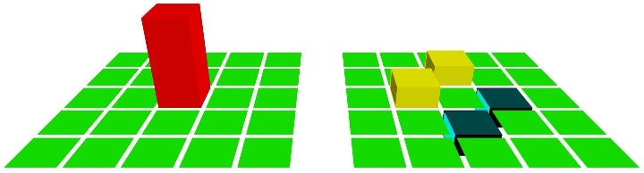
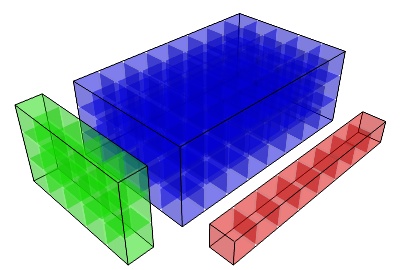
Le broadcasting

Opérations multidimensionelles

• Ajouter un nombre et un tableau marche:

  >>> a = np.ones((3, ))
  >>> a
  array([ 1.,  1.,  1.])
  >>> a + 1
  array([ 2.,  2.,  2.])
  

• Et si on ajoute deux tableaux de forme différentes?

  >>> b = 2*np.ones((2, 1))
  >>> b
  array([[ 2.],
         [ 2.]])
  >>> a + b
  array([[ 3.,  3.,  3.],
         [ 3.,  3.,  3.]])
  

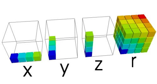
• Les dimensions se complètent:

Pour la performance

• Creation d’une grille 3D

  

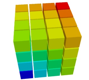
  np.sqrt(x**2 + y**2 + z**2)
  

---

Sans broadcasting:  

>>> x, y, z = np.mgrid[-100:100, -100:100, -100:100]
>>> print x.shape, y.shape, z.shape
(200, 200, 200) (200, 200, 200) (200, 200, 200)
>>> r = np.sqrt(x**2 + y**2 + z**2)

• Temps : 2.3s: création de x, y, z: 0.5s, calcul de r: 1.8s

• Mémoire : 64Mo par tableaux, 6 tableaux, (x, y, z, r) et 2 temporaires

  => 400Mb

• 200^3 opérations élémentaires par opération de tableaux:

  48 million d’opérations.

---

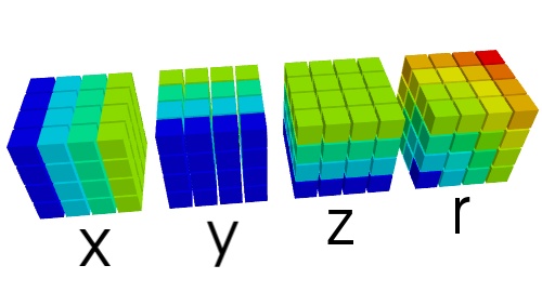
Avec broadcasting:  

>>> x, y, z = np.ogrid[-100:100, -100:100, -100:100]
>>> print x.shape, y.shape, z.shape
(200, 1, 1) (1, 200, 1) (1, 1, 200)
>>> r = np.sqrt(x**2 + y**2 + z**2)

• Temps : 1.1s: création de x, y, z: 6ms

• Mémoire: x, y, z : 1.6Kb. r : 64Mo, et 1 temporaire de 64Mo

  => 120Mb

• 16 million d’opérations

 

numpy: une view structurée sur la mémoire avec des opérations

• données identiques (dtype)
• indexage rapide
• vue/copies
• reshape pas couteux
• opérations comprenant la forme des tableaux